Introduction

Contents/Index

@1. Introduction
2. Using Vector Notation

Linear regression is the task of fitting a linear model/function to some observed values $y$ given some arguments $x$. This task scales to any linear system of equations.

In essence we want to find $\hat{y}$ given some true $y$ and an argument $x$. In order to do this we introduce the squared error as $$ SqrErr = (y_n - f(x_n))^2 $$ Here we have that $\hat{y}_n = f(x_n)$, and that $f$ is linear, that is on the form $$ f(x) = w_1 x + w_0 $$ We can call $w_1$ the weight, and $w_0$ the bias. Here The idea of linear regression is to minimize the squared error hence fitting $f$ as best as possible. We do this by optimizing $w_0$ and $w_1$ on the mean of the squared error. That is $$ argmin_{w_0,w_1} \frac{1}{n} \sum_{n = 1} SqrErr(w_0,w_1) $$ As with any other form of regression we here have an error we want to minimize. We do this by differentiating and solve the result equal to 0. First find the derivative. We rewrite $$ \frac{1}{n} \sum (y_n - f(x_n))^2 = \frac{1}{n} \sum \left [ y_n^2 + f(x_n)^2 - 2y_n f(x_n) \right ] $$ we substitute $f(x)$ with the form it has $$ \frac{1}{n} \sum y_n^2 + (w_1 x_n)^2 + w_0^2 + 2w_1 w_0 x_n - 2y_n (w_1 x_m + w_0) $$ we differentiate, with respect to $w_1$ we get $$ \frac{\partial f}{\partial w_1} = \frac{1}{n} \sum 2w_1 x_n^2 + 2w_0 x_n - 2y_n x_n $$ and with respect to $w_0$ we get $$ \frac{\partial f}{\partial w_0} = \frac{1}{n} \sum 2w_0 + 2w_1 x_n - 2y_n $$ We solve the first derivative equal to 0. Denote $\overline{x}$ as the arithmetic mean of $x$. Denote $\underline{w}$ as the $argmin$ of $w$. We get: $$ 0 = 1/n \sum 2w_1 x_n^2 + 2w_0 x_n - 2y_n x_n \Rightarrow \\ 0 = 1/n \sum w_1 x_n^2 + w_o x_n - y_n x_n \Rightarrow \\ 0 = 1/n \sum (w_1 x_n^2 + \bar{y} x_n - w_1 \bar{x} x_n) - \bar{yx} \Rightarrow \\ 0 = w_1 (\bar{x^2} - (\bar{x})^2) + \bar{y} \bar{x} - \bar{yx} \Rightarrow \\ \underline{w_1} = \frac{\bar{yx} - \bar{y} \bar{x}}{ \bar{x^2} - \bar{x}^2 } $$ We solve the second equal to 0, we get: $$ \underline{w_0} = - \frac{1}{n} \sum w_1 x_n + y_n $$

Example with Python

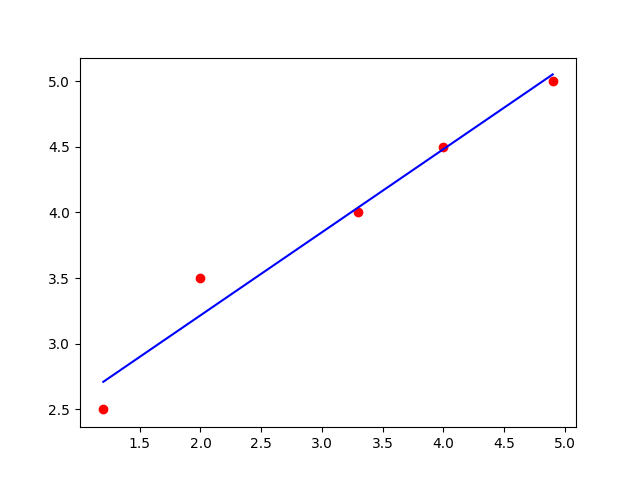
We can do an example in Python3. Given $$ xs = [1.2,2.0,3.3,4.0,4.9] $$ and $$ ys = [2.5,3.5,4.0,4.5,5.0] $$ We define them as numpy arrays and obtain the needed $yx$ and $x^2$ of them. We can then calculate $w_1$ and $w_0$ as thus:

import numpy as np xs = np.array([1.2,2.0,3.3,4.0,4.9]) ys = np.array([2.5,3.5,4.0,4.5,5.0]) yxs = ys * xs xs2 = xs ** 2 # compute using the results of derivative = 0 w1 = (yxs.mean() - ys.mean() * xs.mean()) / (xs2.mean() - xs.mean() ** 2) w0 = ys.mean() - w1 * xs.mean() print("f_model1(x) = " + str(w1) + "x + " + str(w0))

We plot $\hat{y}$ compared to $y$ with the following python code:

y_hat = w1 * xs + w0 plt.scatter(xs,ys,color="red") plt.plot(xs,y_hat,color="blue") plt.show()

Resulting in the plot in Figure 1.

For recording how well the model fits we can use the R squared value. This is computed with the following code

ss_res = ((ys - y_hat) ** 2).sum() ss_tot = ((ys - ys.mean()) ** 2).sum() r2 = 1 - ss_res / ss_tot print("r^2 = " + str(r2))

For which we get $r^2 = 0.965109$. This is a quite high value, meaning the model fits quite well. Which can be seen in the plot.