Multinomial Logistic Regression

Contents/Index

1. Introduction
2. Deriving the model
@3. Multinomial Logistic Regression

We now turn out attention to what is called multinomial logistic regression. The setup is exactly the same as for binary logistic regression, though we now have a label space (or set of classes) of size larger than 2. That is $k \gt 2$. Instead of the sigmoid function we use softmax for activation. In this way we maintain a distribution as output. Now we want to learn $$ p(y = k | x) $$ We have the loss as $$ L_{CE}(\hat{y},y) = - \sum_{1}^{k} 1[y = k] log\ p(y = k | x) $$ Here $1[]$ is an indicator function that returns 1 if the given condition is true and 0 otherwise. The gradient of the loss is given as $$ -(1[y = k] - p(y = k | x)) x_k $$

Implementing multinomial logistic regression in PyTorch

All that theory aside, we can implement this type of regression in PyTorch. Well, we can implement binary logistic regression as well. But let's focus. This setup is exactly the same as a single layer neural network, where the layer is a linear transformation. We want to obtain a function of the form $$ \hat{y} = softmax(w \cdot x + b) $$ that has the least loss with respect to $w$ and $b$.

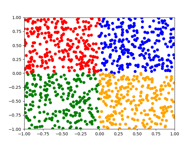
I have devised the following problem I think might be educational: In 2d space place a square with corners $$ (-1,1),(1,1),(1,-1),(-1,-1) $$ We draw/sample points/random variables from this space. We then place a cross in the middle of this space thus dividing the space into 4 squares of the exact same size. That is square 0 has top left corner as $(-1,1)$ and bottom right corner as $(0,0)$. And so on. Now what we want to learn, is the function $f$ that given some point $x = (x_0,x_1)$: $$ f(x) = \begin{cases} 0 & x_0 \lt 0 \land x_1 \geq 0 \\ 1 & x_0 \geq 0 \land x_1 \geq 0 \\ 2 & x_0 \lt 0 \land x_1 \lt 0 \\ 3 & x_0 \geq 0 \land x_1 \lt 0 \end{cases} $$ That is the input has 2 features/dimensions, and the output has 4 classes/dimensions.

We go straight ahead with the code, then we can make a plot that visualizes the problem. We import needed libraries, and then we create the points:

import numpy as np import matplotlib.pyplot as plt import torch as ts import torch.nn as nn import torch.nn.functional as F import torch.optim as optim # this is the only param we optimize on x_size = 1000 x_test_size = 1000 X = np.random.rand(x_size,2) * 2.0 - 1.0 x_test = np.random.rand(x_test_size,2) * 2.0 - 1.0 # these are needed so the plot always has same size plt.xlim([-1.0,1.0]) plt.ylim([-1.0,1.0])

We add $f$ from above along a function that maps labels/classes into some color, this we use for visualization:

def pt2label(x): if x[0] < 0 and x[1] >= 0: return 0 if x[0] >= 0 and x[1] >= 0: return 1 if x[0] < 0 and x[1] < 0: return 2 if x[0] >= 0 and x[1] < 0: return 3 def label2color(l): if l == 0: return "red" elif l == 1: return "blue" elif l == 2: return "green" else: return "orange"

Note that we already have the objective function (the function we want to learn) in terms of python code. What we want to accomplish, is to learn some mathematical representation of this function. We can plot with the following code the inputs/samples:

plt.scatter(X[:,0],X[:,1],c=[label2color(pt2label(pt)) for pt in X]) plt.show()

For which we get the plot as shown i Figure 1.

We next define the PyTorch model along a loss function as follows. Note that we use nn.CrossEntropyLoss which computes both $LogSoftmax$ and obtain the loss in one go.

# the model is just a linear transformation model = nn.Linear(X.shape[1],4) # set the composite loss function loss_fun = nn.CrossEntropyLoss() # choose some optimizer # we do not tinker with the lrate for this example optimizer = optim.SGD(model.parameters(),lr=0.01)

Next we define the training loop. We run the loop once, normally you would run it several times in what is called epochs thus refining the model. Finally we print the average loss for each input point.

avg_loss = 0.0 for pt in X: # reset the gradients model.zero_grad() # convert input point to a tensor # view is needed since the point needs be in 2dim # float() is needed since np rand produces doubles x = ts.tensor(pt).float().view((1,-1)) # convert target to tensor # the target needs not be in 2 dims target = ts.LongTensor([pt2label(pt)]) # compute the result # this is just linear transformation of the input res = model(x) # first do log_softmax on the result # then do negative log loss loss = loss_fun(res,target) # compute all gradients loss.backward() # do a step/steps of size learning rate optimizer.step() # unpack loss with item() and add it to avg avg_loss += loss.item() avg_loss /= X.shape[0] print(avg_loss)

Next we do testing. We want the result to be a plot. We store the label colors in y_test.

y_test = [] with ts.no_grad(): for x in x_test: x = ts.tensor(x).float().view(1,-1) # we do not need to softmax, log-softmax or anything here. l = model(x).argmax() y_test.append(label2color(l)) plt.scatter(x_test[:,0],x_test[:,1],c=y_test) plt.title("x_size = " + str(x_size)) plt.show()

Note that we do not apply $softmax$ to the model when we obtain the label. The output is a one dimensional vector. Softmax turns this into a distribution, but $argmax_{\hat{y}}$ stays the same. Note also that we have 1000 test points. Now we can do different runs adjusting the parameter x_size to have the values $1,10,100,1000,10000,100000$.

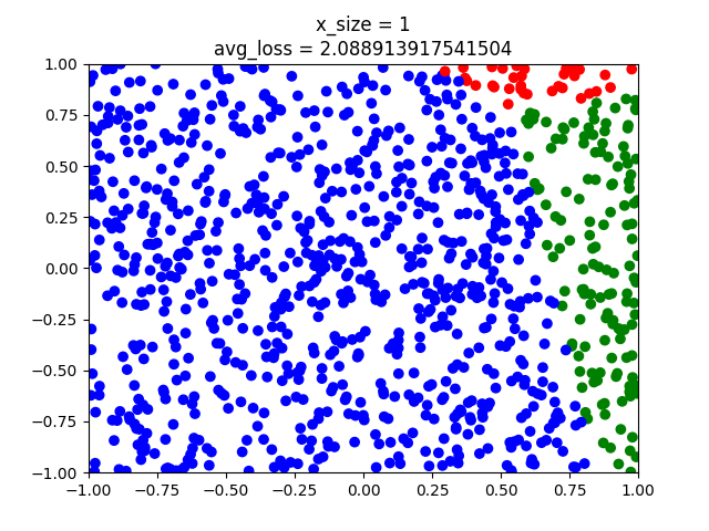
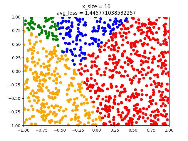
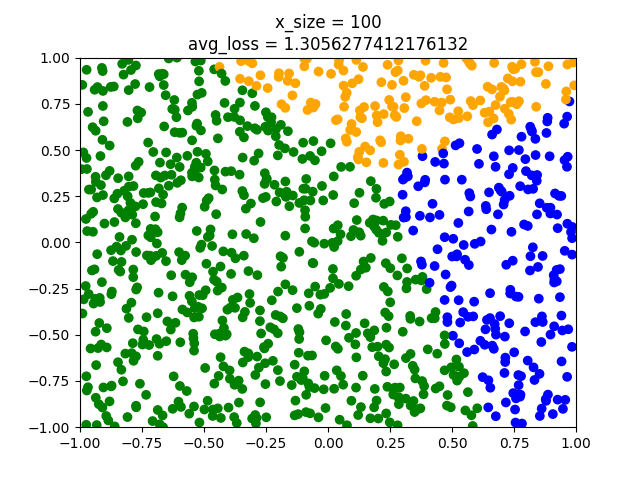
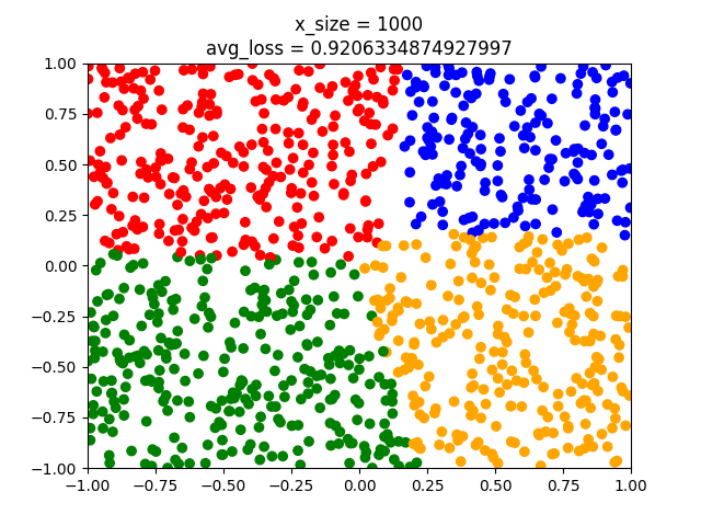
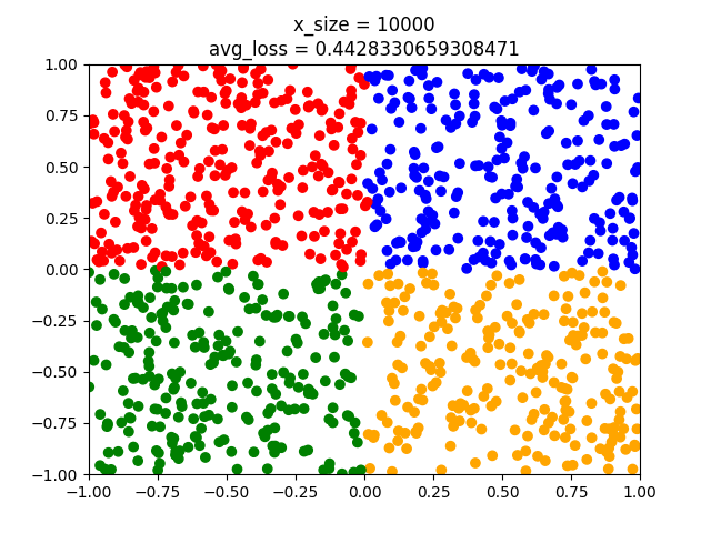
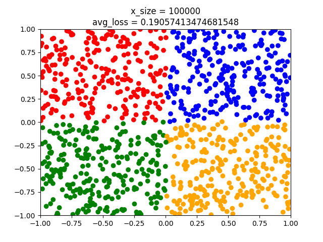
As can be seen the model fits better and better. But even the last model has some points that crosses the classes. When using nn.Linear we initialize with small non-zero random weights. Hence we might have different results from training to training even though we have the same amount of training points. That's why epochs are used.

We can obtain the $w$ and $b$ parameters as follows

print(model.weight) print(model.bias)

For the last model with $10^5$ samples we get

# For w we get Parameter containing: tensor([[-6.8787, 6.8762], [ 6.5487, 6.8114], [-6.8376, -6.5537], [ 6.6465, -6.6249]], requires_grad=True) # For b we get Parameter containing: tensor([0.0672, 0.0527, 0.0541, 0.0419], requires_grad=True)

Which defines $\hat{y}$.

What I think is quite intriguing is that the resulting model is a mathematical representation of a piece of imperative python code. We have learned how to represent some imperative code in terms of a vector and a matrix. This representation shows how the code behaves. pt2label is well defined. But it is defined in python code as a bunch of if-then-else statements. This we now have learned to represent as a mathematical model. It can be shown that a minimal neural network can learn any function. A function needs not be something given in mathematical terms, it can be defined in a programming language. Or it can be a whole program. Another thing is that say I at some point have lost pt2label and have forgotten how it was written. But I might have kept this model. Then I can still model the behavior of the python function without knowing how it works. Thus I have an abstract representation of pt2label in my model.